IFRS 17 close was taking seven hours We brought the reserving cycle down to one
The formulas were not the bottleneck. Late source events, skewed Spark joins and unsafe replays were. I helped turn a 200-million-contract reserving workflow into a repeatable one-hour production cycle without losing its audit trail.
200M
Contracts
30+
Indicators
7h→1h
Reserving Cycle
−40%
Data Issues
Source events arrived late. One product dominated a Spark partition. Actuaries changed assumptions during close. Dozens of dependent calculations still had to produce a result we could trace and rerun.
How to read this case study: Parts 0–2 explain the accounting vocabulary behind the data model. Their formulas are simplified, not a complete accounting specification. Part 3 covers the architecture; Part 4 follows the five production problems and their fixes.
00 · IN BRIEF
The production story in 90 seconds
The reserving workflow covered 200 million contracts. When an assumption changed during close, the replacement result had to appear atomically and remain traceable to its inputs. The timings and incident counts below describe this deployment, not a benchmark for other insurers.
More than 50 Spark jobs shared an event-driven ingestion layer and reusable platform components. We held out-of-order events, avoided row explosion, reused partitioning across calculation windows, detected skew before joins and published replays as atomic snapshots.
Scale
200 million contracts and more than 30 actuarial indicators.
Performance
One production reserving cycle reduced from seven hours to one.
Reliability
Atomic snapshots and rollback kept reruns isolated from readers.
Delivery
Reusable ingestion components moved new actuarial use cases from weeks toward days.
Suggested path: The unresolved limit is in Part 8: snapshot history and rollback did not settle how to handle changing assumptions against a live upstream feed during close.
REFERENCE · CONTEXT
Why the accounting rule became a data-platform problem
Before IFRS17, insurers could carry forward different local accounting treatments for similar contracts. That made results difficult to compare across countries and products.
IFRS17, effective from 1 January 2023, requires insurers to estimate future cash flows, discount them using current assumptions, add an explicit allowance for uncertainty, and recognize profit as insurance service is delivered. Loss-making groups must be identified when they are recognized, with the loss reported immediately in the profit-and-loss statement. Implementing that rule requires far more than a new report: contract grouping, assumption history, repeatable calculations, reconciliations, and evidence that an auditor can trace back to source data.
IFRS4 vs IFRS17, what actually changed
Aspect
IFRS4
IFRS17
Measurement basis
Different local accounting practices could continue.
Risk-adjusted present value of future cash flows, plus unearned profit where applicable.
Discount rates
Treatment depended on the accounting practice retained.
Current measurement; an OCI policy choice affects presentation of insurance finance income or expenses.
Profit recognition
Timing depended on the accounting practice retained.
Profit recognized as insurance contract services are provided.
Onerous contracts
Loss recognized only if liability adequacy test fails at portfolio level.
Tested at group level on day one; loss to P&L immediately, no CSM.
Granularity
Portfolio or product line.
Annual cohorts × profitability buckets, no group spans contracts >12 months apart.
Disclosure
Specified disclosures alongside the accounting practices retained.
Reconciliations explain movements in insurance contract balances and measurement components.
I once watched a CFO realize, mid-quarterly review, that two thirds of his book was technically onerous under the new rule. He went grey. The auditor smiled.
01 · BUILDING BLOCKS
Four values drive the calculation
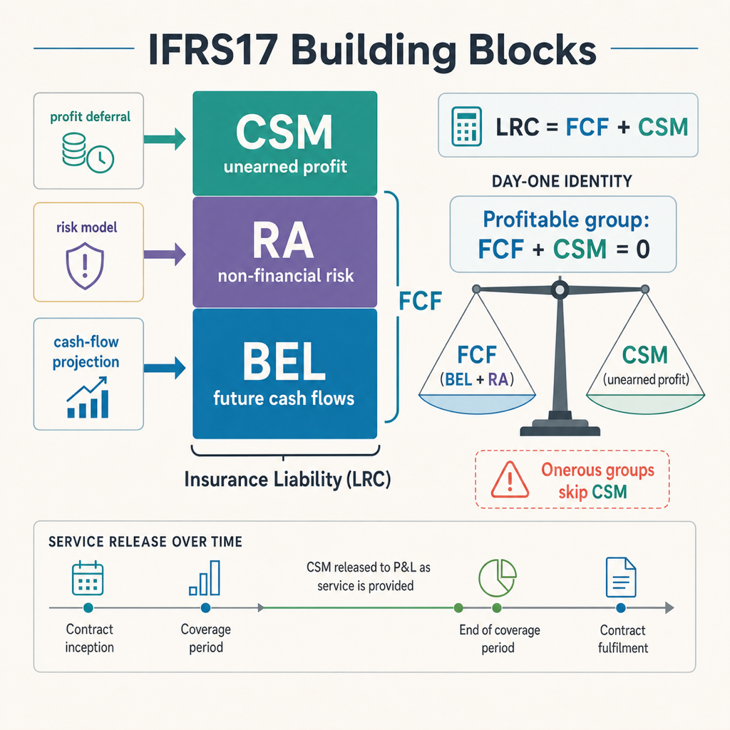
The platform repeatedly computes four values for each group of insurance contracts. The present-value estimate, called BEL in this implementation, captures expected cash flows. RA adds an allowance for non-financial uncertainty. Together they form fulfilment cash flows, or FCF. CSM holds profit that has not yet been earned. At initial recognition, a profitable group satisfies FCF + CSM = 0 under the sign convention used here, so profit is released over the service period instead of being booked on day one.
BEL Best Estimate of Liabilities
BEL = \sum_{t=1}^{T} \frac{E[CF_t]}{(1+r_t)^t}
Probability-weighted present value of every future cash flow, premiums in, claims out, expenses, lapses.
The expected-value core of the liability. No prudence margin baked in; that lives in RA.
RA Risk Adjustment
RA = \mathrm{VaR}_{\alpha}(L) - E[L] \quad \text{or} \quad RA = \mathrm{CoC} \cdot \sum_{t} \frac{SCR_t}{(1+r_t)^t}
Compensation the insurer requires for bearing non-financial uncertainty (mortality, lapse, expense).
Two common implementation approaches are shown. IFRS17 specifies the objective and disclosure, not one mandatory calculation method.
FCF Fulfilment Cash Flows
FCF = BEL + RA
Total economic obligation of the group, before any unearned profit.
Under this implementation's sign convention, negative FCF indicates a profitable group and positive FCF an onerous one.
Unearned profit released over the coverage period as service is delivered.
Eliminates day-one gain. Onerous groups skip CSM and book the loss immediately.
DIAGRAMBuilding blocks stacking up to the insurance liability
The day-one rule
FCF + CSM = 0
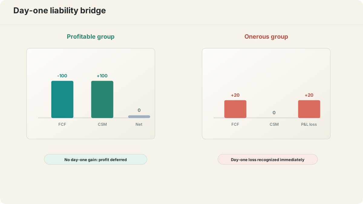
The first time I explained this to a senior actuary, he asked if I was sure. Twice. In the simplified example here, the CSM offsets negative FCF so that the group does not recognize unearned profit at inception. A positive FCF means an initial loss and no CSM. The loss goes to P&L, with a Loss Component in the LRC to track subsequent movements. The full initial-recognition calculation also accounts for cash flows at that date and previously recognized acquisition cash flows; the equation above leaves those details out.
CHARTDay-one liability bridge: profitable vs onerous group
CSM rollforward, how unearned profit moves each period
This term applies to GMM. VFA adjusts for the insurer’s share of changes in underlying-item fair value and related fulfilment cash flows; substituting a current rate in this formula does not model those adjustments.
3
+ New business
+\, CSM_0 \;\text{for new profitable groups}
Only profitable new groups contribute; onerous ones go straight to P&L.
4
± Changes in estimates
\pm\, \Delta FCF_{\text{future service}}
Revised assumptions about future cash flows adjust the CSM. Past-service changes hit P&L.
5
− Amortization
-\, CSM \cdot \frac{CU_t}{\sum_{r \ge t} CU_r}
Amortize using coverage units: sum_assured × survival_probability for life, policies-in-force for non-life.
What lands on the balance sheet
Component
Formula
Contains
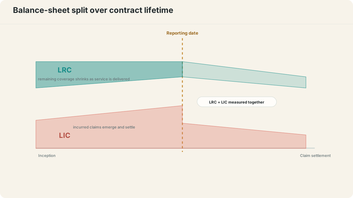
LRC: Liability for Remaining Coverage
LRC = BEL_{RC} + RA_{RC} + CSM
Future-service obligation. Under PAA, measurement follows the standard's simplified approach; it is not generally identical to a legacy UPR minus DAC formula.
LIC: Liability for Incurred Claims
LIC = BEL_{IC} + RA_{IC}
Past-service obligation. Includes IBNR, IBNER and case reserves for events already occurred.
Total insurance liability
\text{Total} = LRC + LIC
The single line on the balance sheet. Both components disclosed separately in the notes.
DIAGRAMBalance-sheet split LRC + LIC over the contract lifetime
Three measurement models, pick the right one
Feature
General (GMM)
Variable Fee (VFA)
Premium Allocation (PAA)
Applicability
All contracts (default)
Direct participation features
Short-term (optional)
Measurement
BEL + CSM + RA
GMM + variable fee adj.
Unearned premium reserve
Revenue
Over life, as risk released
Over life, as risk released
Over coverage period
02 · INDICATORS
The eight indicators the platform uses every day
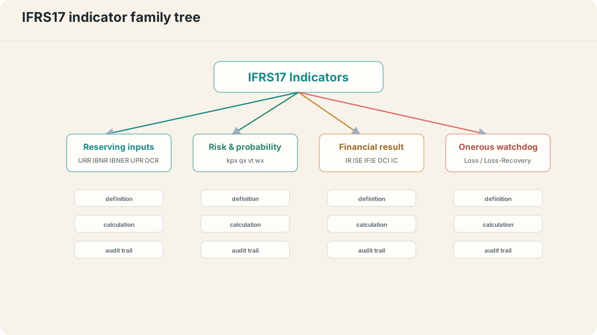
More than thirty indicators fed production reporting at this Tier-1 European insurer. These eight were part of the daily calculation flow, split into the three families feeding FCF, CSM and P&L. The expandable catalogue includes the sensitivities, breakdowns and disclosure subtotals.
DIAGRAMIndicator family tree: 30+ IFRS17 indicators
Reserving inputs (LIC + LRC)
URR
Unexpired Risk Reserve
URR = \max(UPR - DAC,\; UEC)
Held when the unearned premium is insufficient to cover expected claims on the unexpired portion. For death covers: PV(future claims) − PV(future premiums) if recurrent.
Counterpart to IR; together they form the insurance service result.
The rest of the catalog
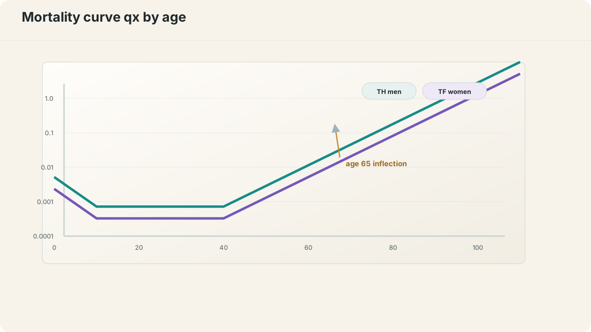
Production reporting also computes IBNER and OCR (reserving), Q(x+t|x) and wx (probability), IFIE, OCI option and IC (financial result). These reuse calculation primitives from the same platform. Their detailed definitions are not needed to follow the architecture in Part 3.
Tracking losses on onerous groups
In the simplified initial-recognition example, FCF > 0 identifies an onerous group. It starts with no CSM; the loss goes to P&L and is tracked through a Loss Component in the LRC. Qualifying improvements in future-service estimates reduce that component before rebuilding a CSM. Loss reversals are excluded from insurance revenue. A Loss-Recovery Component is a separate mechanism for reinsurance contracts held, not the name for a reversal on the underlying insurance group.
03 · ARCHITECTURE
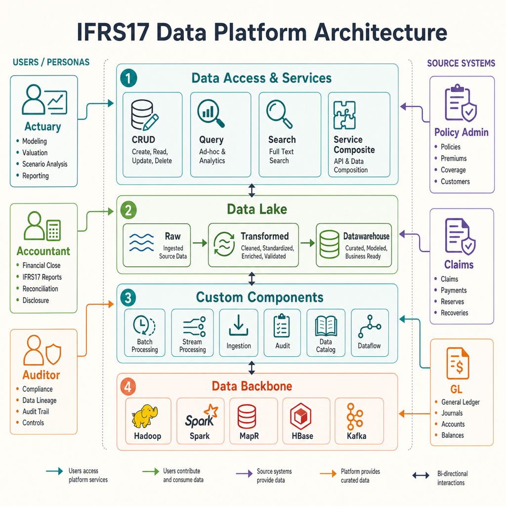
Four layers keep accounting logic separate from distributed systems
The Java/Angular app sat above four layers: service APIs, a three-zone data lake, shared processing components and the distributed data backbone. Stabilizing the interfaces between layers 1 and 4 took six months. At the time it felt like dead weight. Those interfaces later let us replace MapR with vanilla Hadoop without changing the calculations.
DIAGRAMIFRS17 Data Platform: four-layer architecture
The four layers, top to bottom
1. Data Access & Services
Exposes everything below as REST APIs to the Java/Angular web app.
Service Composite Pattern: CRUD Service, Query Service, Search Service.
One stable contract for the front-end. Underlying storage and engine can change without breaking the actuary workflow.
2. Data Lake
Three-zone store: raw landing, transformed, datawarehouse.
Raw data (immutable history), Transformed data (cleansed, conformed), Datawarehouse (actuarial outputs ready for reporting).
Time-travel for audit. Reproducing a 2024-Q3 close means replaying from raw, not patching live tables.
3. Custom Layer Components
Shared tooling for ingestion, processing, audit and data access.
Batch Processing, Stream Processing, Batch Ingestion, Stream Ingestion, Audit Tracking, Data Catalog, Data Auditing, Dataflow Management, Data Exposition.
Squads reuse infrastructure for new actuarial use cases. Generic ingestion components shipped first.
Where the 200M-row joins actually run. Kept invisible from the actuaries, they see Excel-like tables, not partitions.
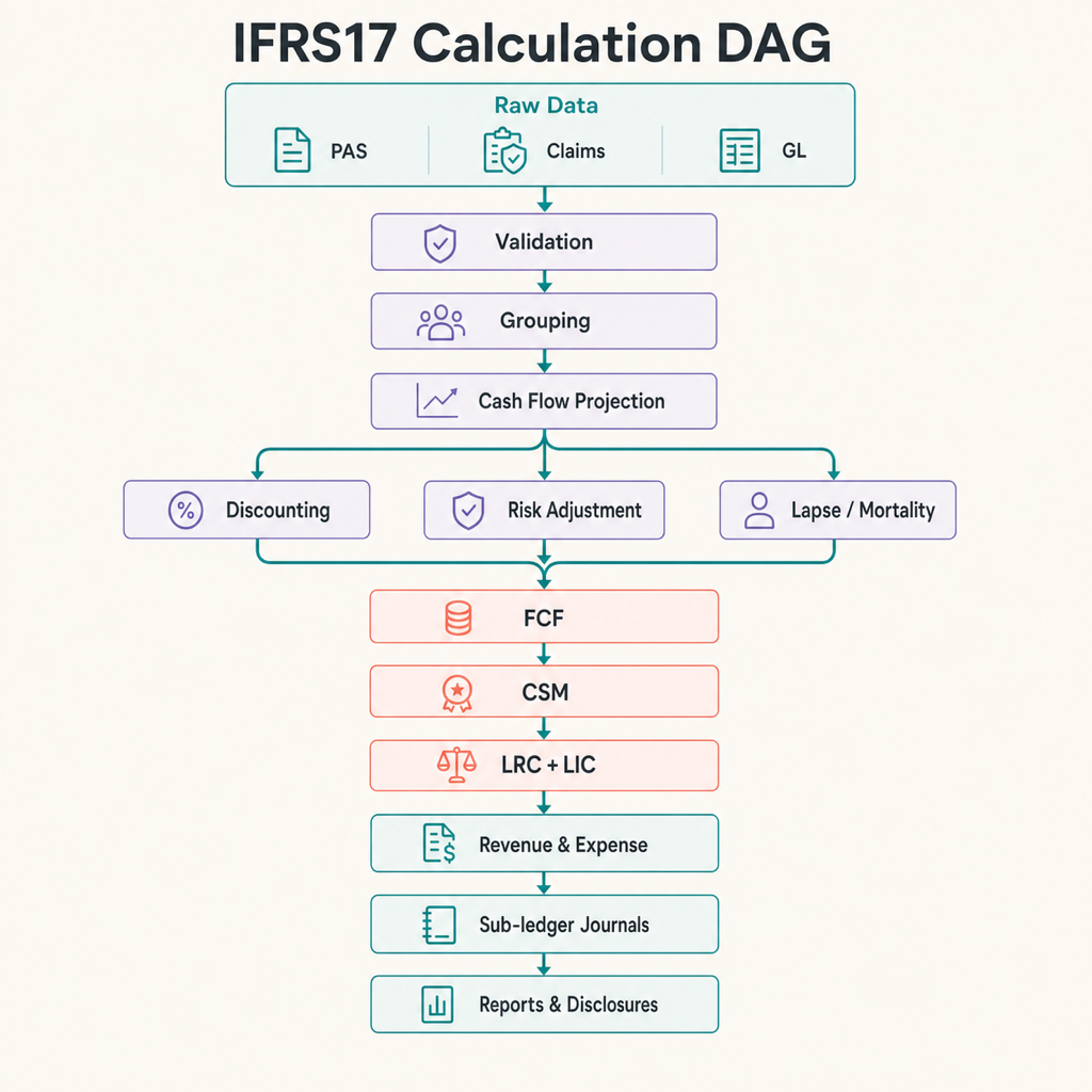
DIAGRAMCalculation dependency graph: 10 steps as a DAG
Calculation dependency graph, 10 steps from raw data to disclosure
Strict topological order. No step skips an upstream dependency, because IFRS17 disclosures must reconcile back to the raw cash-flow projection.
1
Data Ingestion & Validation
Policy admin extracts, claims feeds, asset positions. Schema checks, referential integrity, business-rule gates before anything lands in the lake.
2
Contract Grouping
Portfolio → Profitability bucket → Annual Cohort. The granularity rule that no group spans contracts more than 12 months apart drives the whole partition strategy.
3
Cash Flow Projection per group
Apply the actuarial model: project premiums, claims, expenses period by period over the contract horizon.
4.1
Discounting
Apply the deployment's IFRS17-compliant discount curve. This EU implementation started from EIOPA risk-free data and added a documented illiquidity adjustment.
4.2
Risk Adjustment
Either Cost-of-Capital roll-up of SCR or VaR/CTE on the liability distribution.
4.3
Lapse / mortality assumption application
Multiply projected cash flows by survival, mortality and lapse factors, the behavioural and biometric layer.
5
FCF = PV(CF) + RA
Combine discounted cash flows with the risk adjustment. Negative FCF means profitable, positive means onerous.
6
CSM Calculation
Initial CSM = −FCF₀ for profitable groups. Subsequent periods follow the rollforward: interest, new business, estimate changes, amortization.
7
LRC and LIC assembly
LRC = FCF_RC + CSM. LIC = BEL_IC + RA_IC. The two halves of the insurance liability.
8
Revenue & Expense Recognition
Build IR from CSM amortization, RA release, expected claims released. ISE from incurred claims and onerous losses.
9
Sub-ledger Journal Entries
Translate IFRS17 movements into accounting entries that the general ledger can post without surprise.
10
Reporting & Disclosures
Balance Sheet, P&L, Analysis of Change, CSM/RA/LRC/LIC roll-forwards. Everything must reconcile back to step 1.
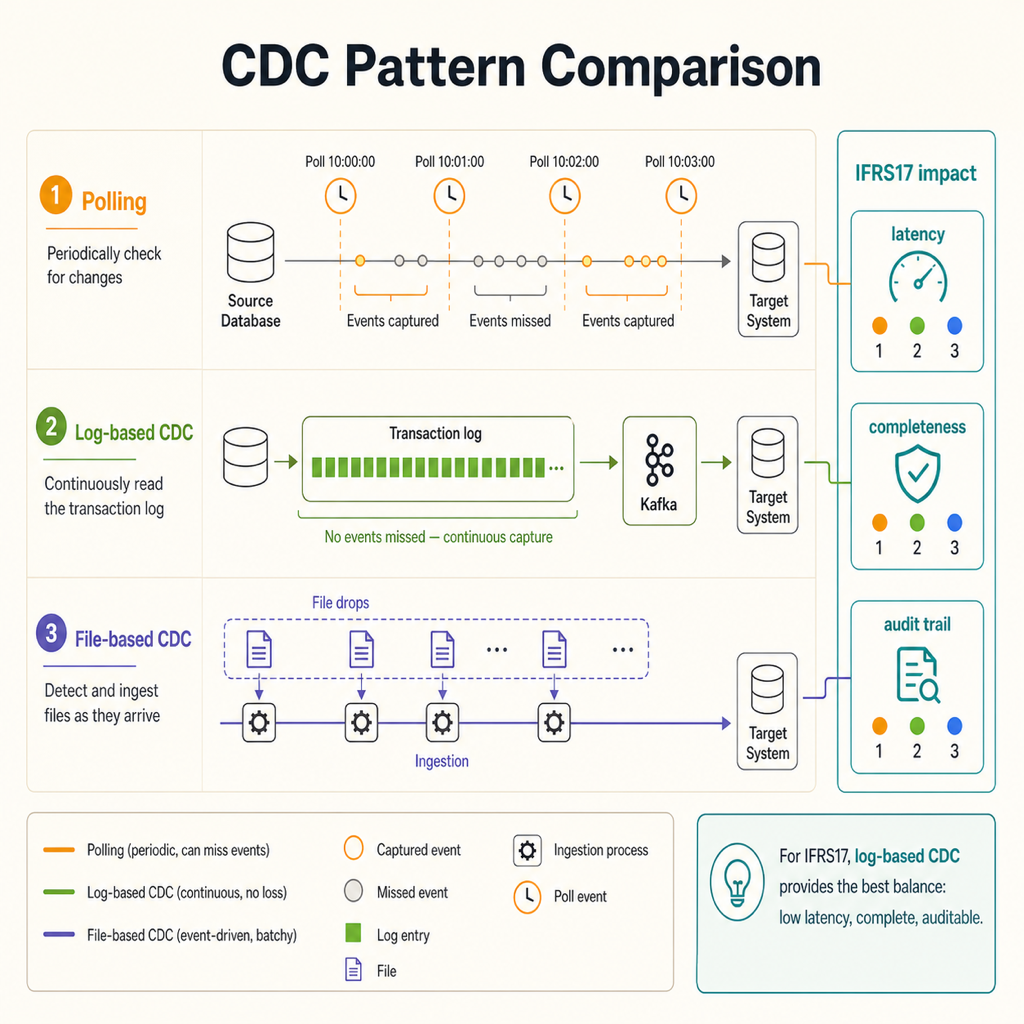
SEQUENCECDC pattern comparison: three timelines side by side
CDC patterns for actuarial data
Polling
Periodic scans for changes. Depending on source history and the polling method, intermediate changes can be missed; scans also add I/O.
Log-Based
Read transaction logs directly when the source exposes complete, ordered change records. Efficient, but not available or appropriate for every actuarial source.
File-Based
Watch the filesystem for actuarial drops. Kafka Connect FilePulse handles the upload pattern actuaries actually use.
Regulatory reporting
Regulator
Scope
Key Role
ACPR
France
French insurance regulator: IFRS17 guidance for the French market
EIOPA
European Union
European insurance supervision and prudential reporting; distinct from IFRS standard-setting
IFRS Foundation
International
Primary standard body: official IFRS17 documentation
04 · WAR STORIES
Five production failures shaped the platform
The main fact table held 200M contracts and joined nightly with reference tables. Changes arrived by CDC from the policy administration system. Spark ran the calculations, Kafka carried events, MapR stored the data and Hadoop YARN managed the cluster. I expected the IFRS17 math to take most of my time. Instead, these five production problems did.
A. 200M-row CDC ingestion with out-of-order events
Problem
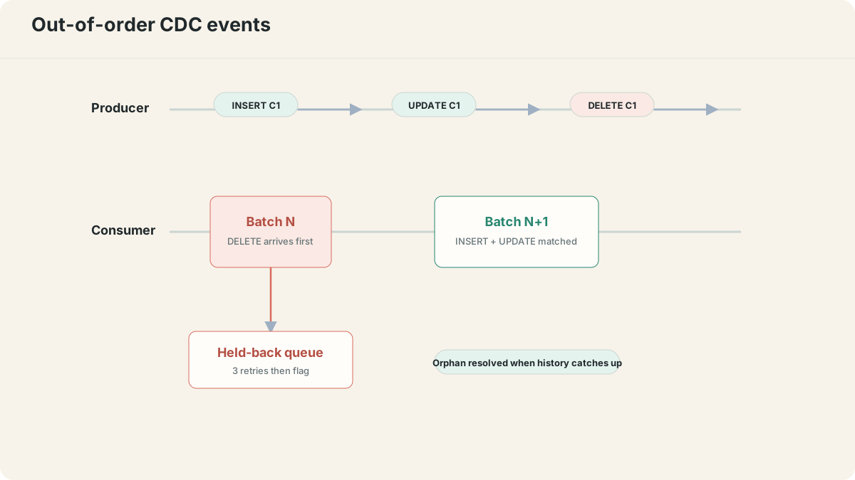
CDC stream from the policy admin sometimes delivered events out of order between micro-batches. A DELETE for a contract would land in batch N, while the corresponding INSERT and UPDATE were still queued for batch N+1. Apply naively and you end up trying to delete a row that does not exist yet, silent orphan, broken reserve calculation downstream.
Root cause
The producer ordered events per partition, but our consumer applied mutations in wall-clock micro-batches. Sorting by event timestamp within a batch did not resolve dependencies on events in another batch. That describes the failure we saw; it does not mean Kafka reordered records within a partition.
Fix
I built an orphan-check stage that ran before applying mutations. Any event with no parent in the warehouse went into a held-back queue on HDFS scratch space. Next batch, the queue was rechecked against the freshly-applied data. Three retries before flagging.
Impact
The observed orphan rate dropped from ~0.4% to zero. Weekend pages from the actuarial team about missing contracts stopped.
SEQUENCEOut-of-order CDC events: DELETE before INSERT
B. Flatmap explosion: contract-month rows kill the executor
Problem
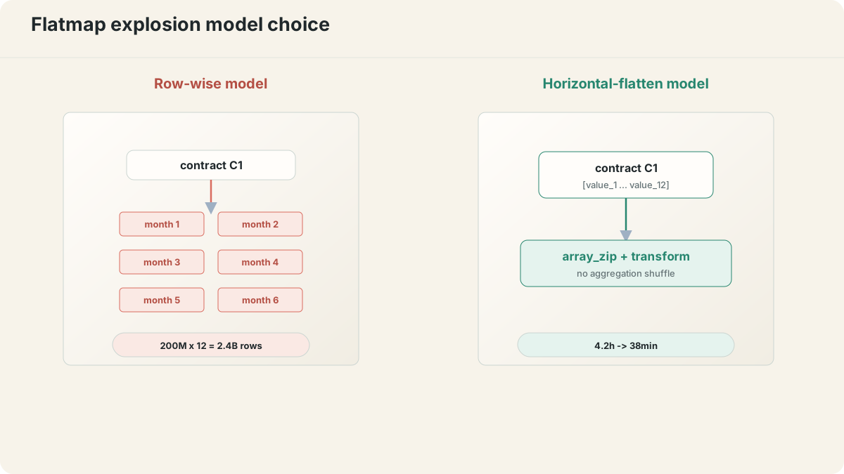
Every contract needs to be projected over its remaining months for cash-flow calculations. The natural shape, one row per contract per month, turns 200M contracts into 2.4B rows when you flatmap over 12 months. Naive partitioning by contract_id triggered massive shuffle on the subsequent groupBy, and a single executor would OOM trying to hold a hot contract group.
Root cause
For this pipeline, expanding periods into rows made each subsequent period-aware aggregation and window more expensive to shuffle.
Fix
Horizontal flatten. Keep one row per contract, store the per-month vector as an array column. Window functions become array_zip + transform. Repartition once by hash(contract_id) % N, write as a bucketed table, sort by (contract_id, period_start). Compatible downstream stages can then reuse that layout instead of repeating the same shuffle.
Impact
Per-contract pipeline went from 4.2 hours to 38 minutes. Memory pressure on executors dropped enough that we cut cluster size by a third.
DIAGRAMFlatmap explosion: row-wise vs horizontal-flatten model
C. Sliding window shuffle on Reserving indicators (URR, IBNR)
Problem
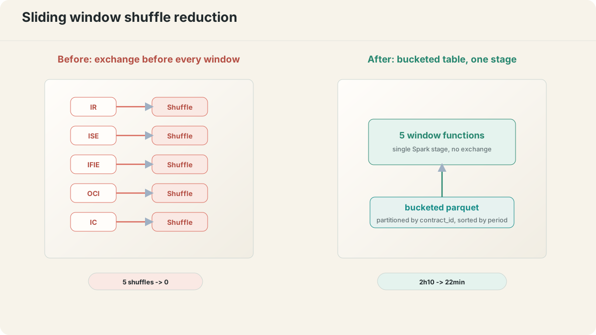
Reserving formulas need rolling windows per contract over development periods. URR = max(UPR − DAC, UEC). IBNR = Ultimate Claims − Paid − Case Reserves, computed at every cut-off. Default Spark partitioning shuffled the whole DAG once per indicator. Five indicators meant five full shuffles of a 200M-row table.
Root cause
Our window specifications needed partitioning and ordering that the input DataFrame did not provide. The execution plans inserted repeated exchanges and sorts.
Fix
Pre-partition by contract_id and sort by (contract_id, period) once at write time using bucketed tables. In this deployment, compatible window specifications then shared a stage and Catalyst elided the exchange when it could reuse the bucket metadata.
Impact
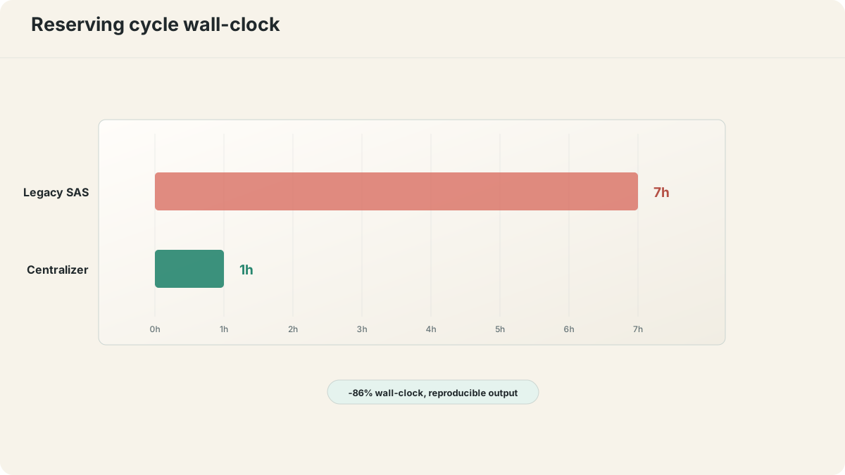
Reserving suite (5 indicators) dropped from 2h10 to 22 minutes. The whole reserving cycle hit the 1-hour target after this fix.
DIAGRAMSliding window shuffle: before vs bucketed table
D. Skewed joins on small reference tables
Problem
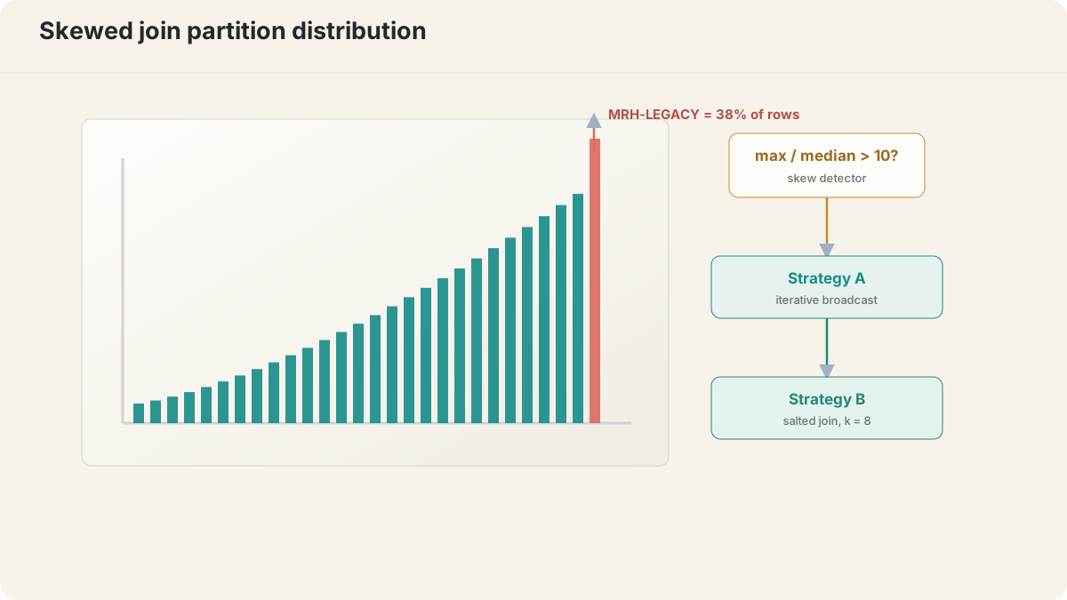
The product reference table had 1,200 codes. One code, the legacy multi-risk household product, accounted for 38% of the fact rows. Joining the fact to the reference table sent that 38% to a single executor, which OOM-ed every time.
Root cause
Hash partitioning put rows with the dominant product code in the same partition. Our Spark configuration did not split that skewed partition.
Fix
I built a skew detector that ran a count-distinct + percentile sketch over partition keys before each large join. If max-partition / median > 10, switch strategy. Path A: broadcast the small side iteratively. Path B fallback: salt the big side with a random key in [0, k), explode the small side k times, join, drop the salt.
Impact
The repeated OOM on this join stopped. The detector caught two more skewed joins later in the year that no one had flagged.
CHARTSkewed join: partition size distribution (power law)
E. Atomic publication and rollback on MapR
Problem
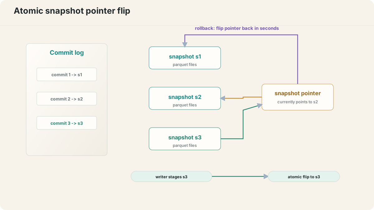
Actuaries reran calculations. A lot. End-of-month close, a parameter changed, replay the last 90 days. We needed atomic commits, either the rerun fully replaced the prior version or nothing changed, and a clean rollback API for when a rerun was wrong. Delta Lake existed but wasn't production-ready on MapR FS at the time.
Root cause
Our Parquet pipeline had no table-level commit protocol. A partial write could expose a mixture of old and new data to readers.
Fix
I built a Dataflow Management Toolkit: an append-only commit log per logical table, a small snapshot-pointer file flipped atomically on commit, snapshot history retained for N days and a manual rollback API that reverted the pointer. Readers resolved through that pointer; writers staged data in a new snapshot directory. Rollback took seconds. This account describes that publication path, not a proof of full ACID behavior under concurrent writers or every crash scenario.
Impact
Actuaries ran 40+ replays a quarter with no split-read incident reported. We documented the pattern on our internal Confluence; three other squads adopted it.
DIAGRAMAtomic snapshot pointer flip for ACID on a data lake
CHARTReserving cycle wall-clock: before vs after the platform
Numbers that mattered to the business
Reserving workflow (one production cycle)
7 hours
→
1 hour
Data quality issues (rolling 90 days post-Catalog launch)
We were replacing SAS and MapR in this deployment with PySpark, Kafka and vanilla Hadoop. Squads needed reusable job structure as well as a new engine. Three patterns covered most of that work.
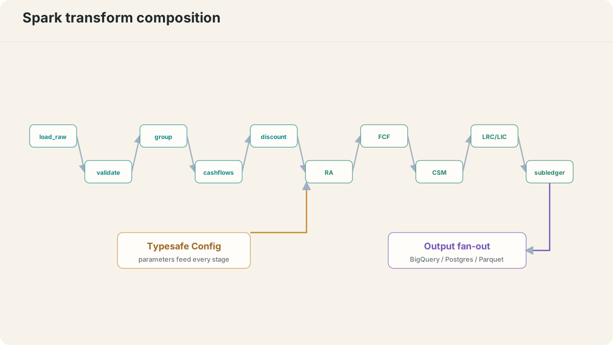
DIAGRAMSpark transform-pattern composition for IFRS17 calculations
Spark Pipeline Frameworks
Orchestrated ETL
MVC-inspired layout. ETL logic out of notebooks, into reusable Python libraries. Fluent interface for composing complex job DAGs.
Transform Pattern
PySpark DataFrame.transform() chained for modular pipelines. Each IFRS17 calculation becomes a composable function.
Configurable Apps
Typesafe Config separates business logic from environment. Same JAR runs in dev, UAT, prod with no code change.
Technology decisions
Area
Technology
Rationale
CDC
MapR-DB CDC API / StreamSets
Native real-time change capture for actuarial pipeline
Orchestration
Airflow / Dagster / Oozie
Airflow: flexible Python DAGs. Dagster: data quality focus. Oozie: Hadoop-native
Data Quality
Deequ (Amazon)
"Unit tests for data": accuracy, completeness, consistency constraints
Serialization
Avro (ingestion) → Parquet (storage)
Avro for write-heavy streaming, Parquet for read-heavy analytics
Migration
hadoop distcp
Standard tool for MapR-FS → HDFS data migration
Security
Kerberos
Authentication for the Hadoop/Spark cluster
SAS → Spark migration
EXL Case Study
EXL reports a 50% improvement in code-migration efficiency for an insurer moving SAS to PySpark. This is a vendor-reported migration result, not a 50% improvement in Spark runtime.
Allianz UK on Databricks
The linked Databricks customer story describes Allianz UK Personal Lines moving from SAS to its Lakehouse. It is a separate migration account, not evidence for this platform’s results.
Hexaware AI-Powered Conversion
Hexaware describes automated SAS-to-PySpark conversion and reports initial conversion accuracy. That does not establish what share of actuarial logic can be migrated without review.
06 · CHEAP CLOUD
Reproduce the calculation flow without production data
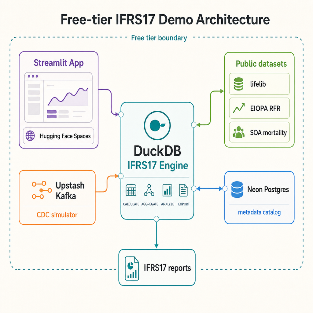
This teaching design uses DuckDB for calculations, Streamlit for the interface, a lightweight event feed to simulate CDC and Postgres for metadata. It is intended for exploring the flow without production customer data. Check the listed free-tier limits before using them. The design is not a validated IFRS17 engine and does not supply production controls, reconciliation, security or close governance.
DIAGRAMFree-tier IFRS17 demo architecture
Component
Tool
Cost
Key Advantages
Calculation Pipeline
DuckDB
Free
In-process, fast OLAP, MIT licensed, embedded in Python
Web App
Streamlit / Gradio
Free
Free hosting on Hugging Face Spaces
CDC Simulation
Upstash Kafka
Free tier
Serverless, pay-per-request, REST API
Metadata Catalog
Supabase / Neon
Free tier
Managed PostgreSQL, ~500MB, branching
07 · ORGANIZATION
Sharing the platform across sixty engineers
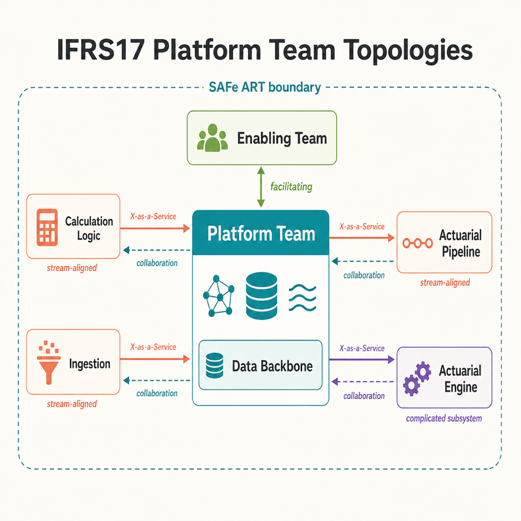
More than 60 engineers across 10 squads worked on the platform. We mapped Team Topologies onto SAFe ARTs to divide responsibility for shared infrastructure, actuarial calculations and ingestion.
DIAGRAMTeam Topologies map for a 60-engineer IFRS17 platform
Team Topologies for Data Platforms
Platform Team
Owns the Data Backbone, Spark, Kafka, MapR/Hadoop. Provides a stable substrate to everyone else. Reduces cognitive load for stream-aligned squads.
Stream-Aligned
Aligned to value streams: IFRS17 calculation, ingestion, actuarial pipeline. End-to-end ownership of one slice.
Enabling Team
Brings new tech and practice into the org, advanced data modelling, fresh stack features, Data Mesh facilitation.
Complicated-Subsystem
Specialists for components that need deep expertise, actuarial calculation engine, regulatory compliance modules.
IDP Success Metrics
Category
Key Metrics
Adoption
Daily active users, % deployments via platform
Developer Experience
Developer NPS, perceived productivity
Delivery Velocity
DORA metrics: lead time, deployment frequency
Reliability
Change failure rate, MTTR
Efficiency
Resource utilization, cloud cost efficiency
Platform Engineering Case Studies
Insurance Company (Microsoft)
An external example of consolidating development workflows through a Backstage internal developer platform.
Financial Institution
An external example of ingestion templates and curated development workflows. The reported reduction from months to days needs a named source before it can serve as a comparison.
Data Mesh Integration
ThoughtWorks pattern: Team Topologies + Data Mesh. Stream-aligned squads own data products (e.g., the IFRS17 actuarial data product). PM + data engineer + analyst in a "product trio".
08 · REFLECTIONS
What I would keep, and what I would replace
After 18 months, I would keep the shared ingestion components and storage adapters. I would move replay controls earlier in the delivery plan and spend less time maintaining a custom table layer.
Three things I'd do the same way
Build the data backbone before the calculation engine.
The first three sprints went into batch processing, ingestion and audit tracking, with no IFRS17 logic. That felt slow. Later squads could reuse those components and onboard in days.
Hide MapR behind generic adapters from day one.
After the MapR FS end-of-life announcement, our move to vanilla Hadoop took four weeks. My estimate without the adapters was four quarters; that comparison was never tested.
Treat the actuaries as users, not consumers.
Weekly syncs with the reserving team, formal RFCs for any pipeline change that affected their close. Bug-bounce-back rate dropped roughly 60% in six months.
Two things I would do differently
Ship the Dataflow Management Toolkit in sprint 1, not sprint 12.
The custom commit-log + snapshot-pointer pattern saved us in production. We built it because Delta Lake wasn't ready on MapR FS, but we waited until reruns started corrupting data. It should have been the first thing built.
Adopt Iceberg or Delta as soon as the platform allowed.
The custom toolkit was the right answer at its moment. Two years later, the OSS table formats had caught up and the home-built layer was a maintenance burden. Migrating off it cost more than building it.
The question I never closed
Deterministic replay when actuaries change assumptions mid-close. We had snapshot history, we had rollback, we could replay from raw, but if the actuary tweaked the lapse curve at 4pm on day-3 of close, the upstream data had already moved. We froze inputs at close start, which papered over the real problem: actuarial close and live data feeds are fundamentally out of phase. Saw the same issue at three other insurers since. Still no clean answer.